It is only just over a century since Einstein in 1905 proved the existence of atoms by predicting the statistical behaviour of suspended particles- until then atoms were just a hypothesis to explain combining ratios in compounds. ( Visualisation of single atoms came in the 1960s with field-ion-microscopes.) Perrin ( 1909) had realised that the continued irregular motion of uniform particles in a suspension, seen in 1827 by Brown for paticles that were small enough but well above molecular size and therefore visible with an optical microscope, indicated the random impacts of the invisible surrounding liquid. Einstein showed how the thermodynamics worked in this situation.
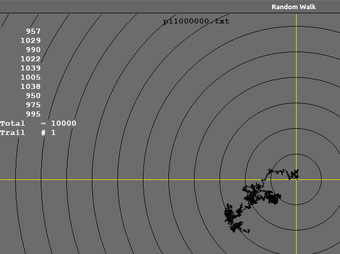
Scenario- imagine a stationary visible particle is surrounded by molecules all rushing around. The impacts will occur from all sides and with an average frequency. What path does the particle follow? I do a 2D simulation, using various ways to get PRNG 'random' digit sequences- one million digits of pi or e downloaded off the internet, or LB4's rnd(), which has known minor flaws. If all impacts pushed it the SAME direction you'd see a straight line going well beyond the screen. But since it does all sorts of zig-zags, curls and other shapes it keeps going back over its own earlier path. Simulating a single particle gives a path in black like this...
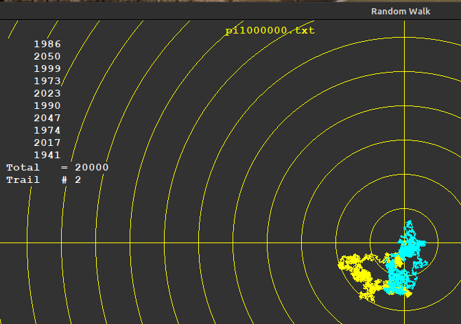
Simulating the particle path a second time, with a different series of random collisions, gives a different path. Coloured differently but one at least partly obscures the other. The number display shows how many times each of the ten directions has been chosen- they will average the same number, but some above and below.
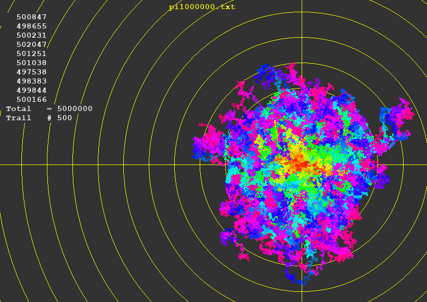
Do this with enough random collisions, and you should get a distribution that is, fuzzily, centred on the start point. Each end point will average sqrt( n) distance. So that you can see the successive paths, I changed the colouring so each path fades from red to magenta using HSV coding. The violet colours will TEND to be most distant from the centre, and the centre tends to red since all routes start there.
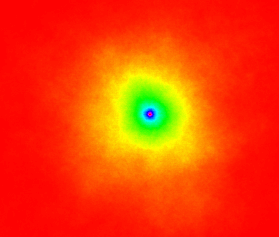
An alternative is to count how many times each point is visited, and represent that as a 'probability density' for the end of each path as a colour plot. Note the scale here is the same- the smaller size is because only a very small proportion of paths go to larger distances.
Various variations of code have been used, including ones to show the LB rnd() bias. The code below is a typical version. I will put up the web pi and e to a million digits on my site- for the LB rnd() version I generate the file in LB.
    nomainwin

    '_______________________________________________________
    'goto [past]
    randomize( 0.99)   '   Run this once to create a re-usable file of LB rnd()
    open "LBrnd1000000.txt" for output as #fO
        for h =1 to 1000000
            v       =int( 10 *rnd( 1))
            #fO str$( v);
        next h
    close #fO
  [past]
'-----------------------------------------------------------

    global pi, col$: pi   =4 *atn( 1)

    dim d( 10)

    data "LBrnd1000000.txt"    '   LB rnd()
    'data "pi1000000.txt"    '    web Pi
    'data "rand1000000.txt"   '  web random

    WindowWidth     =1220
    WindowHeight    = 800

    stride          =   1

    open "Random Walk" for graphics_nsb as #wg

    #wg "trapclose quit ; font courier_new 12 bold"


    for b =1 to 1   '   3
        read f$

        open f$ for input as #fI
            L            =lof( #fI)
            rnd1000000$  =input$( #fI, L)
        close #fI

        #wg "backcolor 50 50 50"
        #wg "color yellow ; goto 610 325 ; down ; fill 50 50 50 ; line 610 0 610 700 ; line 0 325 1220 325"
        #wg "up ; goto 350 20 ; down"
        #wg "\"; f$

        x   =610
        y   =325

        #wg "up ; goto "; x; " "; y
        #wg "down"
        for k =50 to 700 step 50
            #wg "circle "; k
        next k

        #wg "flush"
        #wg "color yellow"

        for trail =1 to 2'500
            start =int( 990000 *rnd( 1))    '   start anywhere that gives a run of 10000

            for i =1 to 10000
                v       =val( mid$( rnd1000000$, start +i, 1))
                d( v)   =d( v) +1
                dirn    =v *36 *pi /180
                x       =x +stride *cos( dirn)
                y       =y +stride *sin( dirn)
                'call hsv2rgb int( i /30) mod 360, 0.99, 0.99    '   hue, saturation, value
                '#wg "color "; col$
                #wg "goto "; int( x); " "; int( y)
                scan
            next i

            #wg "up ; goto 20 40 ; down ; color white"
            tot     =0

            for j =0 to 9
                #wg "\ " +using( "########", d( j))
                tot     =tot +d( j)
            next j

            #wg "\ Total   = " +str$( tot)
            #wg "\ Trail   # "; trail

            #wg "flush ; getbmp scr 1 1 1220 800 ; cls ; drawbmp scr 1 1"

            x   =610
            y   =325
            #wg "place "; x; " "; y
            #wg "color cyan"
        next trail

        #wg "flush ; getbmp scr 1 1 1220 800"
        bmpsave "scr", "BrownianPath" +word$( f$, 1, ".") +str$( time$( "seconds")) +".bmp"
    next b

    wait

    sub quit h$
        close #h$
        end
    end sub


    sub hsv2rgb h, s, v '                       hue 0-360, saturation 0-1, value 0-1
        c   =v *s       '                           chroma
        h   =h
        x   =c *( 1 -abs( ( ( h /60) mod 2) -1))
        m   =v -c   '                               matching adjustment

        select case
            case h < 60
                r = c: g = x: b = 0
            case h <120
                r = x: g = c: b = 0
            case h <180
                r = 0: g = c: b = x
            case h <240
                r = 0: g = x: b = c
            case h <300
                r = x: g = 0: b = c
            case else
                r = c: g = 0: b = x
        end select

        rd      = abs( int( 256 *( r + m)))
        gn      = abs( int( 256 *( g + m)))
        bu      = abs( int( 256 *( b + m)))
        col$    =right$( "  " +str$( rd), 3) +" " +right$( "   " +str$( gn), 3) +" " +right$( "   " +str$( bu), 3)

    end sub