2-Dimensional Diffraction- FFT in 2D
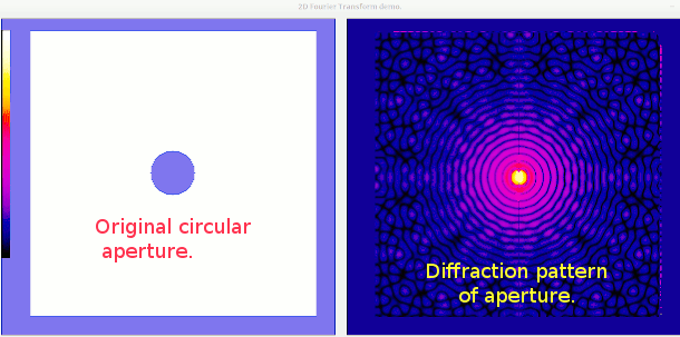

In my student days we didn't have lasers to give coherent monochromatis light. It was still magic to be able to flip from frequency domain to real world. The beauty of the images, and the rapidly developing application of X-rays to crystallography were very attractive to me. A year or two later and I built a mains powered He-Ne gas laser. Now we can buy high-intensity solid-state laser cheaply on the 'net.
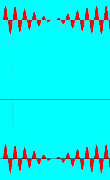
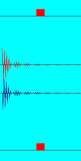
The screen shots below show the analysis and re-synthesis of four waves.
Beats shows 'sin 30 +sin 33'. Pulse is a low mark/space rectangular wave. Square wave approximation was generated from the known series of terms.
 . .
. .  . .
. . 
Example LB code- uses a supplied colour-scale.
    '   ***********************************************************
    '   **                                                       **
    '   **  1DFFT.bas       27/02/2017       tenochtitlanuk      **
    '   **                    beats                              **
    '   ***********************************************************


    global n, pi                    '   globally available pi, number of data values- a multiple of 2-

    n       =1024
                                    '   globally available real and imaginary data for main and sub sections
    dim realData( n), imagData( n)  '   the FFT operates in-place, changing the data to its transform.

    pi      =   4 *atn( 1)

    WindowWidth  =1080
    WindowHeight = 720

    nomainwin

    open "FFT demo." for graphics_nsb as #wg

    #wg "trapclose quit"
    #wg "goto 20 100 ; down ; size 1 ; fill cyan ; color white"

    for i =1 to n
        'if i >508 and i <516 then realData( i)  =1 else realData( i)  =0.05
        for k = 1 to 3 step 2
            realData( i) =realData( i) +1 /k *sin( i /n *k *10 *2 *pi)
        next k
        imagData( i)  =0
        #wg "color red      ; line "; 20 +1024 *i /n; " 80 "; 20 +1024 *i /n; " "; 80 -int( 25 *realData( i))
    next i

    call fft -1 '   ie compute FFT not inverse-   1 for fwd FFT, -1 for reverse

    #wg "size 5"
    for i =1 to n ' but symmetrical on x axis so really only want left-hand half.
        #wg "color red      ; line "; 20 +1024 *i /n; " 250 "; 20 +1024 *i /n; " "; 250 -int( 0.18 *realData( i))
        #wg "color darkblue ; line "; 20 +1024 *i /n; " 350 "; 20 +1024 *i /n; " "; 350 -int( 0.18 *imagData( i))
    next i

    call fft 1  '   ie compute inverse

    #wg "size 1"
    for i =1 to n ' but symmetrical on x axis so really only want left-hand half.
        #wg "color red      ; line "; 20 +1024 *i /n; " 550 "; 20 +1024 *i /n; " "; 550 -int( 25 *realData( i))
    next i

    #wg "color black ; up ; goto 10 80 ; down ; goto 1034 80"

    for v =250 to 550 step 100
        if v <>450 then #wg "up ; goto 10 "; v; " ; down ; goto 1034 "; v
    next v

    wait

    sub fft isi
        j   =1
        for i =1 to n
            if i <j then call exchangeTerms i, j
            m   =n /2
            while j >m
                j   =j -m
                m   =int( ( m +1) /2)
            wend
            j   =j +m
        next i

        mmax    =1

        while mmax <n
            istep   =2 *mmax
            for m =1 to mmax
                theta   =pi *isi *( m -1) /mmax
                wr      =cos( theta)
                wi      =sin( theta)

                for i =m to n step istep
                    j               =i +mmax
                    tempr           =wr *realData( j) -wi *imagData( j)
                    tempi           =wr *imagData( j) +wi *realData( j)
                    realData( j)    =realData( i) -tempr
                    imagData( j)    =imagData( i) -tempi
                    realData( i)    =realData( i) +tempr
                    imagData( i)    =imagData( i) +tempi
                    scan
                next i
            next m

            mmax    =istep
        wend

        if isi =-1 then exit sub    '   else normalise values

        for i =1 to n
            realData( i)  =realData( i) /n
            imagData( i)  =imagData( i) /n
        next i
    end sub

    sub exchangeTerms i, j
        temp            =realData( i)
        realData( i)    =realData( j)
        realData( j)    =temp

        temp            =imagData( i)
        imagData( i)    =imagData( j)
        imagData( j)    =temp
    end sub

    sub quit h$
        close #h$
        end
    end sub


    '                       ***********************************************************
    '                       **                                                       **
    '                       **   2DFourier11.bas       05/03/2017    tenochtitlanuk  **
    '                       **                       beats                           **
    '                       ***********************************************************


    nomainwin

    global n, pi                    '   globally available pi, number of data values- a multiple of 2-
    n            = 128
                                    '   globally available real and imaginary data for main and sub sections
    dim realData( n), imagData( n)  '   the FFT operates in-place, changing the data array to its transform.
    dim imageArray$( n, n)          '   holds R and I values as a csv string
    dim ColLookUp$( 256)

    pi           =   4 *atn( 1)

    UpperLeftX   =  10
    UpperLeftY   =  10
    WindowWidth  =1300
    WindowHeight = 700

    graphicbox #w.gb1,   20, 10, 600, 570
    graphicbox #w.gb2,  640, 10, 600, 570


    open "2D Fourier Transform demo." for window as #w

    #w     "trapclose quit"
    #w.gb1 "down ; fill 40 40 180 ; size 1 ; color darkgray"
    #w.gb2 "down ; fill 40 40  40 ; size 1 ; color darkgray"

    loadbmp "scr", "colRange.bmp"
    #w.gb1 "drawbmp scr 0 20 ; size 1"

    gosub [fillColLookUp]
    gosub [initImageArray]

    for row =1 to n
        for col =1 to n   '   copy a row of data to array for computing its FFT
            realData( col)    =val( word$( imageArray$( row, col), 1, ","))
            imagData( col)    =val( word$( imageArray$( row, col), 2, ","))
        next col

        call fft -1

        for col =1 to n   '   do FFT and copy back to image array
            imageArray$( row, col)   =str$( realData( col)) +"," +str$( imagData( col))
            amp                      =amp( ( realData( col)^2 +imagData( col)^2)^0.5)      '   int( 100 *log( 1 +( realData( col)^2 +imagData( col)^2)^0.5))
            #w.gb2 "backcolor "; ColLookUp$( amp)
            #w.gb2 "color     "; ColLookUp$( amp)
            call sqDraw 2, row, col
        next col

    next row

    call screenGrab "X"

    for col =1 to n
        for row =1 to n         '   copy a row of data to array for computing its FFT
            realData( row)          =val( word$( imageArray$( row, col), 1, ","))
            imagData( row)          =val( word$( imageArray$( row, col), 2, ","))
        next row

        call fft -1

        for row =1 to n
            imageArray$( row, col)   =str$( realData( row)) +"," +str$( imagData( row))
            amp                      =amp( ( realData( row)^2 +imagData( row)^2)^0.5)      '   int( 100 *log( 1 +( realData( row)^2 +imagData( row)^2)^0.5))
            #w.gb2 "backcolor "; ColLookUp$( amp)
            #w.gb2 "color     "; ColLookUp$( amp)
            call sqDraw 2, row, col
        next row

    next col

    'call screenGrab "Y"
    wait

    sub screenGrab i$
        for x =0 to 256 step 256
            for y =0 to 256 step 256
                #w.gb2 "getbmp scr "; x +50; " "; y +20; " 256 256"
                bmpsave "scr", i$ +str$( x) +str$( y) +".bmp"
            next y
        next x
    end sub

    sub fft isi
        j   =1
        for i =1 to n
            if i <j then call exchangeTerms i, j
            m   =n /2
            while j >m
                j   =j -m
                m   =int( ( m +1) /2)
            wend
            j   =j +m
        next i

        mmax    =1

        while mmax <n
            istep   =2 *mmax
            for m =1 to mmax
                theta   =pi *isi *( m -1) /mmax
                wr      =cos( theta)
                wi      =sin( theta)

                for i =m to n step istep
                    j               =i +mmax
                    tempr           =wr *realData( j) -wi *imagData( j)
                    tempi           =wr *imagData( j) +wi *realData( j)
                    realData( j)    =realData( i) -tempr
                    imagData( j)    =imagData( i) -tempi
                    realData( i)    =realData( i) +tempr
                    imagData( i)    =imagData( i) +tempi
                    scan
                next i
            next m

            mmax    =istep
        wend

        if isi =-1 then exit sub    '   else normalise values

        for i =1 to n
            realData( i)  =realData( i) /n
            imagData( i)  =imagData( i) /n
        next i
    end sub

    sub exchangeTerms i, j
        temp            =realData( i)
        realData( i)    =realData( j)
        realData( j)    =temp

        temp            =imagData( i)
        imagData( i)    =imagData( j)
        imagData( j)    =temp
    end sub

  [fillColLookUp]
    handleg     =hwnd( #w.gb1)
    calldll #user32, "GetDC", handleg as ulong, hDC as ulong

    x   =5

    for M =0 to 255 '   0 =white up to 255 =black
        y               =int( 22 +410 *M /256)
        calldll #gdi32, "GetPixel", hDC as ulong, x as long, y as long, pixcol as ulong

        bl              = int(  pixcol /( 256*256))
        gr              = int( (pixcol               -bl *256*256) / 256)
        re              = int(  pixcol               -bl *256*256           - gr *256)

        ColLookUp$( 255 -M)  =str$( re) +" " +str$( gr) +" " +str$( bl)

    next M

    callDll #user32, "ReleaseDC", handleg as ulong, hDC as ulong, result as void

  return

  [initImageArray]  '   fill image array with data- here a single central item
    for x =1 to n
        for y =1 to n
            r =( (x-n/2)^2 +(y-n/2)^2)^0.5
            if r <20 then
                imageArray$( y, x) ="0.2,0"
                #w.gb1 "backcolor "; ColLookUp$(   0)
                #w.gb1 "color     "; ColLookUp$(   0)
            else
                imageArray$( y, x) ="0,0"
                #w.gb1 "backcolor "; ColLookUp$( 255)
                #w.gb1 "color     "; ColLookUp$( 255)
            end if

            call sqDraw 1, y, x
            scan
        next y
    next x
  return

    function amp( i)
        amp =int( 40 *log( 1.1 +i))
    end function

    sub sqDraw w, row, col '   row is down y axis, col along x axis
        select case n
            case 64
                dd =8
            case 128
                dd =4
            case 256
                dd =2
        end select

        if w =1 then
            #w.gb1 "up ; goto ";        50     +dd *col; " ";     20 +dd *row
            #w.gb1 "down ; boxfilled "; 50 +dd +dd *col; " "; 20 +dd +dd *row
        else
            #w.gb2 "up ; goto ";        50     +dd *col; " ";     20 +dd *row
            #w.gb2 "down ; boxfilled "; 50 +dd +dd *col; " "; 20 +dd +dd *row
        end if
    end sub

    sub quit h$
        close #h$
        end
    end sub


Code will be up shortly as a 2D_FFT.zip